It's safe to say that knowing the ins and outs of Excel is essential for a profession as data-oriented as accounting. If used correctly, Excel can make your job infinitely easier, and can help you save time and brain power. Becker has compiled our top three tips that are easy to implement in an Excel workbook, and that can help you work quickly and more efficiently!

Tip #1
Unique function

Every accountant knows about the filter function, which can help sift through a large range of data - but did you know that you can use the UNIQUE function to return all unique values from a given list? Here’s how!

*NOTE – this trick will only work for Microsoft Windows Insider accountholders – you can join the community for free on Microsoft’s website.

1. For a given set of data, create a table - to do so, select the desired data and use the keystroke combination CONTROL + T.

2. As shown in Figure 1 and the worksheet UNIQUE of this Excel workbook, we made the range B4:B9 into a table (named, “people.”) If we add a new name (say, “Rebecca”) to cell B10, then the formula =UNIQUE(people[Names]) in cell E4 will automatically populate cell E9 with “Rebecca,” as this is a new, unique value in our list. You now have a list of entirely unique values from a given set of data! How easy was that? Hang on to this file – you’ll need it for Tip #3!

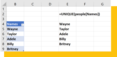
Figure 1: The UNIQUE formula

Tip #2
Writing a formula across sheets

During busy season, every minute counts. You’ll need every tip and trick to get a spare minute, which will help you tremendously during crunch time when deadlines are around every corner. One simple way to save time? Streamlining your Excel sheet setup! If you need to set up multiple Excel sheets with the same formula in each (say, for fiscal year planning), here’s a quick technique to help you copy your setup across worksheets.

This workbook contains a blank worksheet for the months January-June and a blank summary worksheet. Suppose we want each of our monthly worksheets to track units sold, price, and revenue in the cell range B1:B3.

To copy your setup across all sheets, follow these easy steps:

1. Click on the January worksheet tab and hold down the Shift key and click on the June tab.

2. Fill in cells A1:A3 of the January worksheet as shown in Figure 2, with data for units, price and revenue. Enter numbers in cells B1 and B2, but in cell B3, enter the formula ‘=B1*B2’.

3. After clicking on the summary worksheet (this will undo the selection of the January-June worksheets), you will find that each month’s worksheet looks like Figure 2 - voilà! With this trick, you’ll be able to avoid copying and pasting your worksheet multiple times.

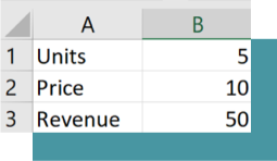
Figure 2: Copying formulas across multiple sheets

Tip #3
Using pivot tables without refresh

Ever make a pivot table and need to add additional data? Us, too! There’s a simple way to add even more data into a pivot table and to have your formulas update to include this newly added data. This is especially helpful for tasks where you need to continually account for new data as you receive it.

Use this workbook to get started – it’s the same workbook as in Tip #1! Here is how to do it:

1. Start on the worksheet “Pivot Table.” In cell F16, the formula =UNIQUE(sales[Product]) will return a list of all products.

2. In cell G15, the formula =TRANSPOSE(UNIQUE(sales[Country])) returns a list of all countries.

3. Enter in cell G16 the (AMAZING) formula =SUMIFS(sales[Revenue],sales[Product],F16#,sales[Country],G15#) This will compute all the needed totals - you don’t even need to copy the formula! The F16# and G15# portions of the formula ensure that total revenue is computed for each product-country combination.

4. Amazingly, if new data is entered starting in row 211, revenue for any new product-country combination will be totaled. For example, in row 211 of the worksheet “Pivot Table,” we entered a revenue of 2000 for Chip 12 in Mexico. As Figure 3 shows, our formulas will automatically include this data in the calculations.

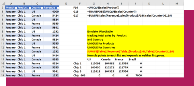
Figure 3: Refreshed pivot tables

Other quick tips!

That’s not all! Here are a few other handy Excel tips that you can use to help format and organize your spreadsheets the way you want, with just a clack of a few keys:

• Create a table
  CONTROL + T
  This keyboard shortcut turns a range of data into a table for easy access to sorting!

• Auto-fit columns
  CONTROL + A
  to select all text, then hold down ALT + H + O + I
  This sequence allows you to select all of the text in a given sheet, and auto-fit columns to this text (or data) - no more manually adjusting column width!

• Conditional formatting
  ALT + O + D
  Select the text you want to format, then use these keystrokes to create new conditional formatting rules - color coding, anyone?

• Add today’s date
  CTRL + ;
  In a given cell, the control button held down with the semicolon key will enter today's date, so you don’t have to open your calendar app!

• Format cell options
  CTRL + 1
  This sequence will pull up available formatting for text, including currency, dates and more.

We hope these techniques have helped you become an Excel wizard and make your workdays a little bit easier. Learn more of Becker’s best-kept Excel secrets with our Microsoft Excel Fundamentals + Data Analytics Certificate.