Dynamic Ranges and the OFFSET function

Microsoft Excel offers a world of time-saving tools for accounting professionals. Whether you’re a CPA at a public firm, a CMA increasing efficiency for your company, an Enrolled Agent managing your clients’ tax compliance, or any type of accounting or finance expert; leveraging Excel is an essential skillset that improves your productivity and effectiveness on the job. 

The OFFSET function is just one of the important Excel tools to improve your projects. 

What is the OFFSET function in Excel? 

Excel’s OFFSET function is a formula that finds a cell or range of cells, starting from a reference point and moving a certain number of rows or columns. 

The function makes it easy to navigate your Excel file and find specific data, and—in more complex projects—helps you quickly create dynamic ranges and calculations that automatically update as you update your original data.¹

Defining each variable of the OFFSET function 

Understanding the OFFEST formula is key to knowing how it works and how best to use it in your spreadsheets. 

To use the OFFSET function, type this formula in Excel:

 OFFSET(cell reference, rows moved, columns moved, height, width)

Each one of these values means: 

1. Cell reference: The cell providing a position from which you want to start the search 
2. Rows moved: The number of rows you want to move in the search, starting from the “cell reference.” 
   1. “Rows” can be a positive or negative number: a positive number counts down from the “cell reference,” a negative number counts up. 
3. Columns moved: The number of columns you want to move in the search, starting from the “cell reference.” 
   1. “Columns” can be a positive or negative number: a positive number counts to the right from the “cell reference,” a negative number counts to the left. 
4. Height: [Optional] The number of rows (going up) that you want to include in the returned value of the formula. This must be a positive number. 
   1. If you choose not to include a “height” value, the default return is one row. 
5. Width: [Optional] The number of columns (going to the right) that you want to include in the returned value of the formula. This must be a positive number.  
   1. If you choose not to include a “width” value, the default return is one column.² 

For example, you may have an OFFET function formula written like this: 

= OFFSET(G1, 3, -1) 

In this example, the formula begins at the reference cell, G1. Then, it moves 3 rows down and one column to the left. Since there are no inputted values for “height” and “width,” the formula will return the contents of only one cell: F4. 

How to use the OFFSET function 

The previous example shows the OFFSET working in its simplest form. However, when you’re managing a spreadsheet of large, complex data, you’ll use the OFFSET function to perform much more complicated and time-saving purposes.

Here, we’ll walk through how to use the OFFSET function to: 

1. Return the last number in a column, even as you add new data 
2. Create dynamic ranges that update automatically when new data is added 
3. Create a chart that always charts only the last 6 months of sales 

Returning the last number in a column 

To show how you write a formula that always returns unit sales during the most recent month (even when new data is added), we’ll use the example worksheet, “Most recent” (see Figure 1).

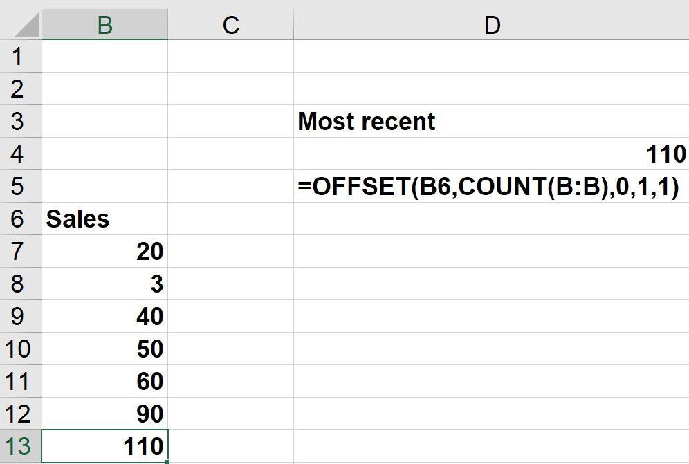
^{Figure 1: Returning the last number in a column} 

In this example, Column B contains monthly unit sales of a product. In cell D4, we entered the OFFSET function formula, “=OFFSET(B6,COUNT(B:B),0,1,1)” 

The key to this formula is the quick trick: “COUNT(B:B).” This shortcut will always return a count of the number of numerical entries in Column B. Currently, COUNT(B:B) = 7, so our formula moves 7 rows below cell B6 (or cell reference) and returns the value of 110 from cell B13. 

If we input another month of sales into cell B14, then the new COUNT(B:B) will equal 8, so our formula will return the new number from cell B14. 

Creating a dynamic range 

The worksheet Dynamic Range (see Figure 2) shows the sales of three products for each of our nine salespeople. From this data, we want to create a named range that automatically updates whenever new data is added beginning in column A and/or row 1.

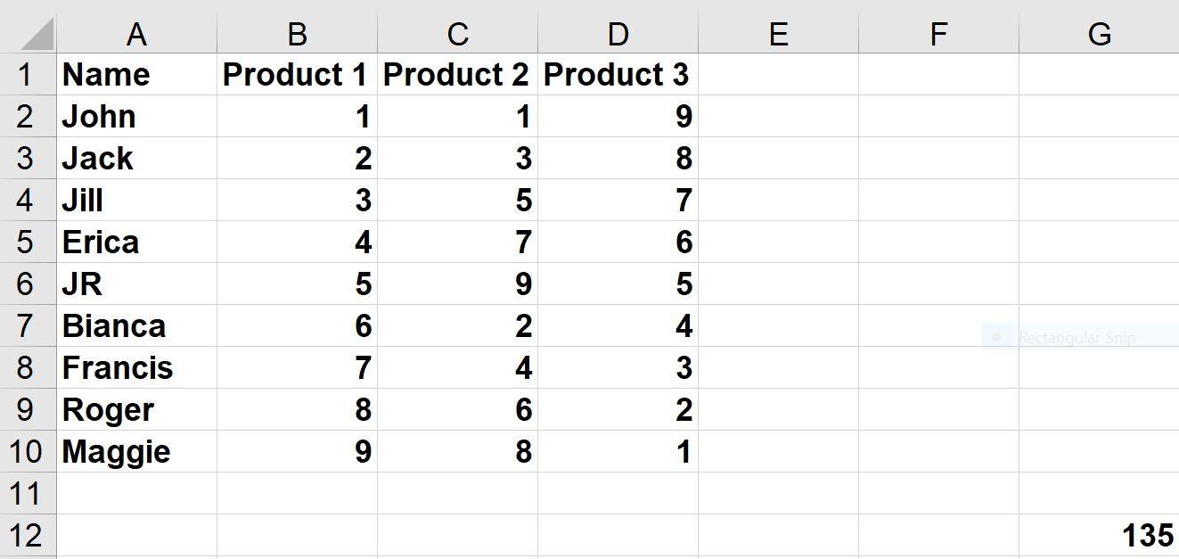
^{Figure 2: Creating a dynamic range}
 

In the Excel Formulas Tab, click “Define Name” to create a range name based on a formula (in our case, the OFFSET function). It is important to get the dollar signs right in this formula; Excel will copy it as you move around the spreadsheet.

To create the desired dynamic range, click on “Define Name” in the “Formulas” tab at the top of your spreadsheet. 

1. Enter a name (we chose “Data”) 
2. In the “Refers to” portion of the dialog box, enter the formula (preferably by pointing to cells) 

The formula may look like this:  

=OFFSET(‘Dynamic Range’!$A$1,0,0,COUNTA(‘Dynamic Range’!$A:$A),COUNTA(‘Dynamic Range’!$1:$1))

This formula creates a range that always starts in cell A1. You can affirm this by seeing that $A$1 carries the dollar signs. 

The COUNTA function counts all non-blanks in a range, entire row, or entire column. Here the COUNTA(‘Dynamic Range’!$A:$A) portion of the formula counts the number of rows containing data in Column A. This gives us the desired height of the dynamic range. 

The portion of the formula = COUNTA(‘Dynamic Range’!$1:$1) counts the number of columns containing data in Row 1. This gives us the width of the desired range. 

In cell G12, the formula =SUM(data) returns the sum (135) of all the numbers in the range A1:D9. 

To show that our named range is indeed dynamic, you could add a name to cell A11 followed by data in B11:D11. You could likewise add Product 4 data to column E. Your formula in cell G12 will automatically update your SUM formula to include the newly added data. 

Creating a chart that returns the last 6 months of sales 

To create a chart that always shows only the last 6 months of sales, we used formulas to create two dynamic ranges(see Figure 3): 

• The range Months: OFFSET(‘Last 6’!$A$3,COUNT(‘Last 6’!$A:$A)-5,0,6,1)  
• The range Sales : OFFSET(‘Last 6’!$B$3,COUNT(‘Last 6’!$A:$A)-5,0,6,1)

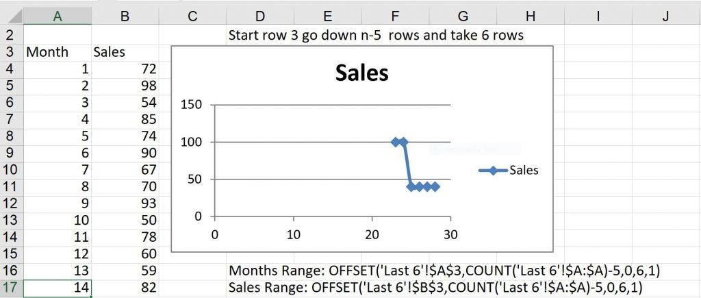
^{Figure 3: Chart returning the last 6 months of sales}

The range, “Months” contains 6 cells in column A. This range contains six months: months 23-28, located in rows 26-31.

Similarly the range, “Sales” currently returns B26:B31. 

To create our dynamic chart, first select all the data (the range A3:B31) and then create a scatter chart with lines and markers. Click on your data and in the “Formula” bar, you will see this formula: 

= SERIES(‘Last 6′!$B$3,’Last 6′!$A$4:$A$31,’Last 6’!$B$4:$B$31,1) 

To create a dynamic chart, replace the ranges in this formula by our dynamic range names. You will now see this formula: 

= SERIES(‘Last 6′!$B$3,’Last 6′!months,’Last 6’!sales,1) 

Add new data and you will see that the chart always shows only the last 6 months of sales! 

Download our FREE ebook Excel automation for accountants 

With step-by-step tutorials and real world examples, learn valuable automation functions in Excel that save time, improve accuracy, and and enhance your skills!

Download your free guide

Learn more with Excel CPE 

These ways to use the OFFSET function reveal just the tip of the iceberg when it comes to all you can do in Excel. Become an Excel expert through your CPE learning, saving yourself time, increasing your productivity, and reducing the chance of typos or missed data. 

Becker’s Microsoft® Excel Fundamentals + Data Analytics Certificate equips you with all the essential knowledge that every accounting professional needs to make game-changing moves in Excel. 

And if you’re looking for even more CPE in Excel and beyond, our Prime CPE subscription includes unlimited access to premium courses, webcasts, and CPE podcasts—so you can enhance your knowledge and complete CPE with flexibility and convenience.