

Microsoft Excel now has 14 new functions that make it easier to manipulate text within spreadsheets. Excel text functions can be used to display text and numbers in a more readable format – especially valuable when you’re presenting a spreadsheet to a client.
In this article, you’ll learn how to use each of Excel’s newest text functions and be provided with easy-to-follow examples. The workbook NewTextFunctions.xlsx contains our work.
Download our FREE ebook Excel automation for accountants
With step-by-step tutorials and real world examples, learn valuable automation functions in Excel that save time, improve accuracy, and and enhance your skills!
How to use Excel text functions
Below, we’ll demonstrate how to use each of the newest text functions in Excel. Figure 1 illustrates the use of the TEXTAFTER, TEXTBEFORE, TEXTSPLIT, VSTACK, and HSTACK functions.
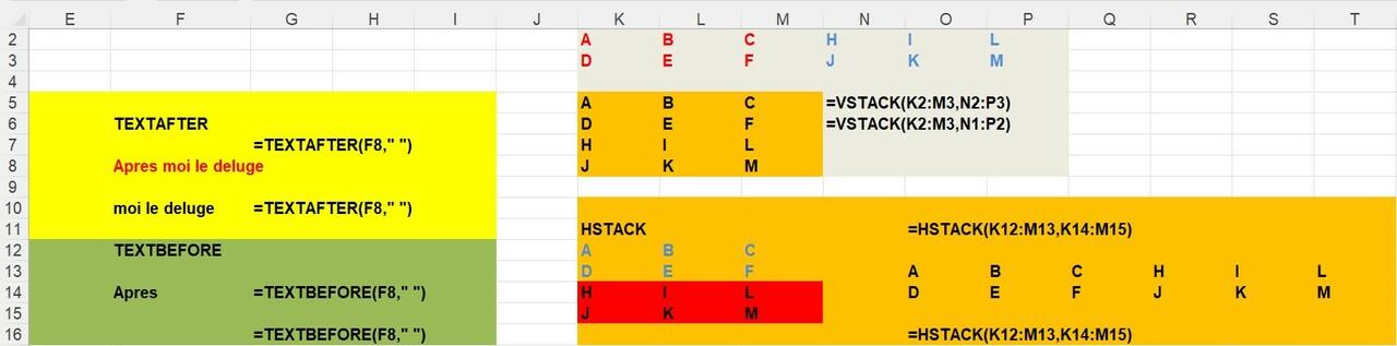
Figure 1 Examples of TEXTBFORE, TEXTAFTER, TEXTSPLIT, VSTACK and HSTACK functions
- TEXTAFTER function
The TEXTAFTER function extracts the text string from a cell that occurs after the first occurrence of a delimiter. For example, the formula =TEXTAFTER(F8," ") returns everything occurring after the first space in “Apres moi le deluge” (Louis XIV’s famous quote in which he declared, “after me, the deluge.”) The result in cell F10 is “moi le deluge.”
- TEXTBEFORE function
The TEXTBEFORE function extracts the text string from a cell that occurs before the first occurrence of a delimiter. For example, entering the formula =TEXTBEFORE(F8," ") in cell F14 returns “Apres” in cell F14.
- TEXTSPLIT function
The TEXTSPLIT function “splits” the contents of a cell (across multiple cells) at each occurrence of a delimiter. For example, entering the formula =TEXTSPLIT(F8," ") in cell F22 enters “Apre,” “moi,” “le” and “deluge” in separate cells. This is much better than TEXT to COLUMNS, because TEXTSPLIT will update if the original cell changes, while TEXT to COLUMNS will not.
- VSTACK function
The VSTACK function stacks two (or more) arrays on top of each other. For example, entering the function = VSTACK(K2:M3,N2:P3) in cell K5, stacks the array
ABC
DEF
On top of the array
HIL
JKM.
- HSTACK function
The HSTACK function horizontally stacks two (or more) arrays into one array. For example, entering the formula = HSTACK(K12:M13,K14:M15) in cell O13 yields
ABCHIL
DEFJKM.
Figure 2 illustrates the use of the TOROW and TOCOL functions.
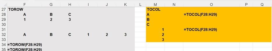
Figure 2 Examples of TOROW and TOCOL functions
- TOROW function
The TOROW function transforms an array into a single row. For example, the formula =TOROW(F28:H29) in cell F32 transforms
ABC
123
into ABC123.
- TOCOL function
The TOCOL function transforms an array into a single column. For example, the formula = TOCOL(F28:H29) in cell M28 transforms
ABC
123
into
A
B
C
1
2
3.
Figure 3 illustrates the use of WRAPROWS and WRAPCOLS functions.
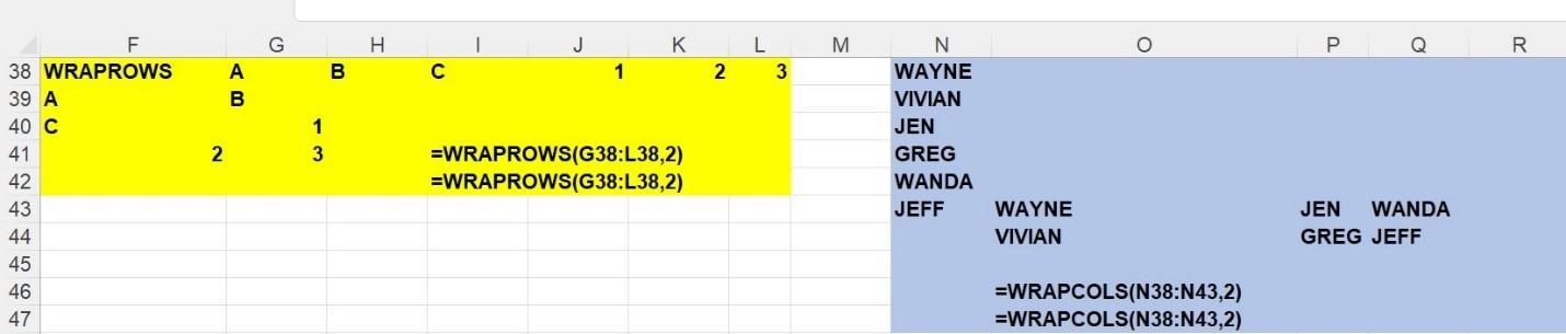
Figure 3 Examples of WRAPROWS and WRAPCOLS functions
- WRAPROWS function
The WRAPROWS function transforms a row into a designated number of rows. For example, the formula =WRAPROWS(G38:L38,2) in cell F39 transforms
| A | B | C | 1 | 2 | 3 |
into rows each containing two columns. The result is
| A | B |
| C | 1 |
| 2 | 3 |
- WRAPCOLS function
The WRAPCOLS function transforms a column into a designated number of rows. The formula =WRAPCOLS(N38:N43,2) in cell O43 transforms
| WAYNE |
| VIVIAN |
| JEN |
| GREG |
| WANDA |
| JEFF |
into columns each containing two rows. The result is
| WAYNE | JEN | WANDA |
| VIVIAN | GREG | JEFF |
Figure 4 illustrates the use of the TAKE, DROP, CHOOSEROWS and CHOOSECOLS functions.
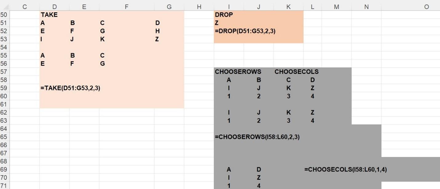
Figure 4 Examples of TAKE, DROP, CHOOSEROWS, and CHOOSECOLS functions
- TAKE function
The formula =TAKE(D51:G53,2,3) in cell D55 “takes” the first two rows and first three columns of the array
| A | B | C | D |
| E | F | G | H |
| I | J | K | Z |
yielding
| A | B | C |
| E | F | G |
- DROP function
The formula =DROP(D51:G53,2,3) in cell I51 drops the first 2 rows and first 3 columns from the array.
| A | B | C | D |
| E | F | G | H |
| I | J | K | Z |
The result is
Z.
- CHOOSEROWS function
The formula = CHOOSEROWS(D51:G53,1,3) in cell I58 chooses rows 1 and 3 from the array
| A | B | C | D |
| E | F | G | H |
| I | J | K | Z |
The result is the first and third rows of the initial array.
| A | B | C | D |
| I | J | K | Z |
- CHOOSECOLS function
The formula = CHOOSECOLS(I58:L60,1,4) in cell I69 returns the first and fourth columns of the following.
| A | B | C | D |
| I | J | K | Z |
| 1 | 2 | 3 | 4 |
The result is the first and fourth columns of the initial array.
| A | D |
| I | Z |
| 1 | 4 |
And finally, Figure 5 illustrates the use of the EXPAND function.
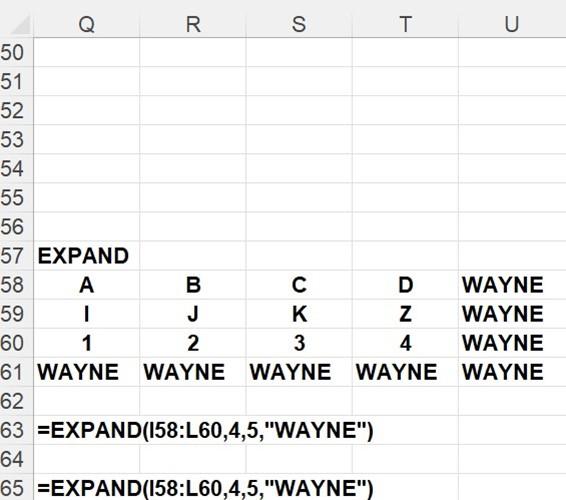
Figure 5 Example of the EXPAND Function
- EXPAND function
The formula = EXPAND(I58:L60,4,5,"WAYNE") in cell Q58 expands the array
| A | B | C | D |
| I | J | K | Z |
| 1 | 2 | 3 | 4 |
to 4 rows and 5 columns by padding the array with cells containing “WAYNE”. The result is the following.
| A | B | C | D | WAYNE |
| I | J | K | Z | WAYNE |
| 1 | 2 | 3 | 4 | WAYNE |
| WAYNE | WAYNE | WAYNE | WAYNE | WAYNE |
Uses for Excel text functions
Why should you learn these text functions in Excel? They are incredibly versatily and can be used in a variety of ways to manipulate and analyze text data. The most common uses include:
- Data cleaning: Trim, Clean, and Substitute can remove unwanted spaces, non-printable characters, and replace specific text which is needed to prepare data for analysis.
- Text extraction: Left, Right, and Mid extract specific parts of a text string like the doman from an email address or characters from a product code.
- Text conversion: Upper, Lower, and Proper can change the case of text to standardize your text data.
- Concatenation: Concat or TextJoin allows you to combine several text strings into one to create full names from first and last names or address components.
- Text location: Use Find, Search, and Replace functions to help locate specific text within a string and replace it with new text.
- Formatting numbers as text: The Text function formats numbers and dates as text in a specific format to create custom date formats or adding leading zeroes to numbers.
All these uses can make your data more organized and easier to analyze, saving you time in your work.
Learn more with Excel CPE
Excel offers a wide variety of functions, formulas, and automation that can save you hours of work while improving accuracy and outcomes. To help you make the most out of this software, we offer a wide variety of CPE courses to support your learning!
Check out Becker's wide range of CPE courses that teach you to make the most of this powerful tool:
- Excel: Technical Analysis Trading Strategies
- Excel: Enterprise Risk Management
- Excel: Magic with Excel
- Excel: Solve Hard Problems in Corporate Finance
- Excel Metrics: Best Practices
- Python for Excel Users: A Gentle Introduction
These and many more Excel-focused, CPE credit-earning courses are included in Becker's Prime CPE subscription. Sign up now for 12 months of access to over 1700 on-demand, webcast, and podcast CPE courses!
Unlock Unlimited CPE with a Prime Subscription
Becker makes it easy to meet your CPE requirements, gain new skills, and stay aware of critical updates and changes in the industry!
With Prime, you can access over 1,700 courses for a full year and earn unlimited CPE credits.
Related Articles


Share


