

Conditional formatting in Excel allows you to automatically format cells based on specific criteria or rules that you define. Instead of manually formatting cells based on changing data, you can set up conditions that will format the cell automatically, making it easier to identify patterns or exceptions in your data. While you can specify formatting based on conditions, you can also leverage a conditional formatting formula and formula-based customization rules.
We're providing a step-by-step guide to using conditional formatting with a formula so you can enhance how you manage, analyze, and present financial data while saving time!
How to implement a conditional formatting formula in Excel
To implement a conditional formatting formula in Excel, follow these steps:
- Select the range where the formatting will be applied.
- Select CONDITIONAL FORMATTING from the HOME tab on the top ribbon
- Select NEW RULE from the drop down menu
- Select USE A FORMULA and enter your into the FORMAT VALUES WHERE THIS FORMULA IS TRUE
- Select FORMAT
Conditional formatting with a formula walkthrough
We created a sample walkthrough to help you see exactly how to complete this process using information related to an example real estate company. In this example, we want to create a conditional formatting formula that will subtract the original price of a property from the sale price, and highlight cells with where the selling price was above the original listing price as green.
First, we highlighted the area to apply the formatting which was J2 through J100. From there, we chose CONDITIONAL FORMATTING under the HOME menu on the top ribbon and choose NEW RULE from the drop-down menu.
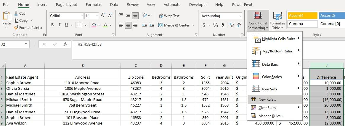
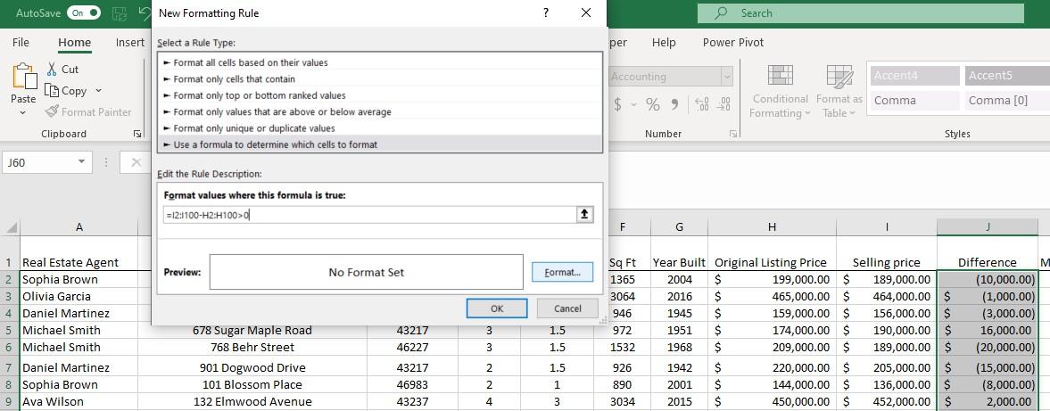
After clicking on NEW RULE, a new box is visible, and we chose USE A FORMULA TO DETERMINE WHICH CELLS TO FORMAT.
Below, we entered the conditional formatting formula =I2:I100-H2:H100>0 and then choose FORMAT. Note, there is already a formula applied to column J subtracting column I from column H to determine the difference.
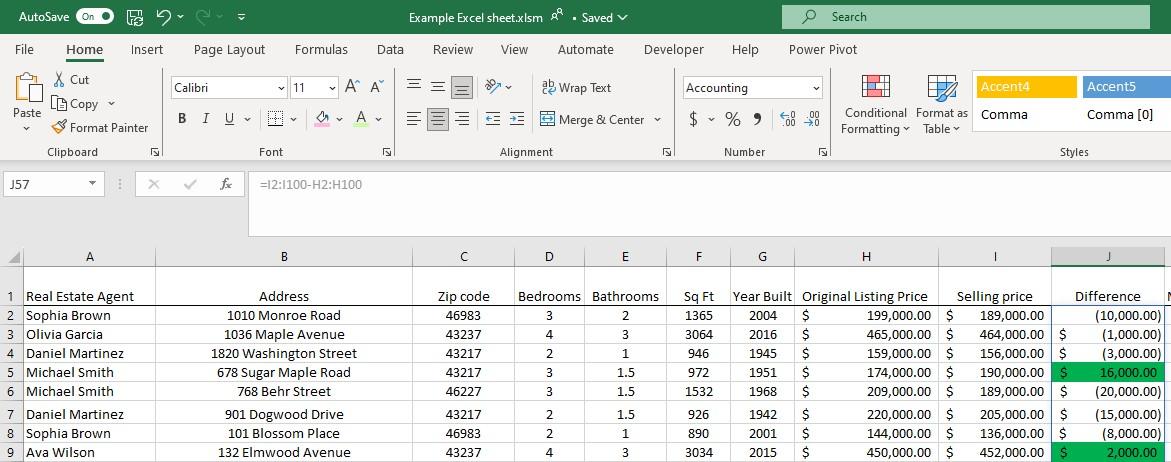
In the format screen, we chose green to highlight sales numbers over zero and clicked OK. We were returned to the screen above with the preview of the formatting. Then we selected OK again. The result is any existing numbers above zero will automatically have a green highlight.
Learn how to use a conditional formatting formula in Excel
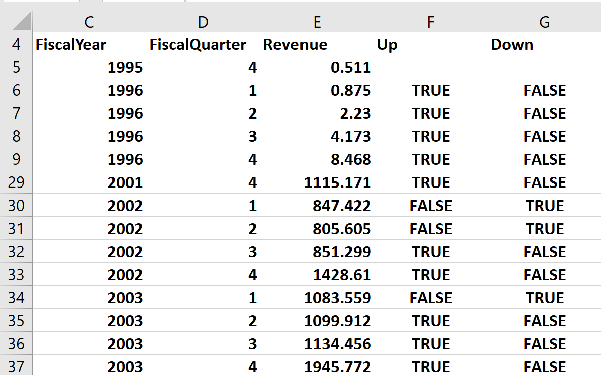
Ready to try it? In the file Beckerfeb2020.xlsx, we demonstrate how to use a conditional formatting formula using a formula capability. In this Excel spreadsheet, we're using quarterly revenues from Amazon in Column E (in millions of dollars). Each line demonstrates the next quarter's revenue. We want to easily see when revenue increases or decreases from quarter to quarter and can easily do this through conditional formatting with a formula.
To begin, we select the cell range E6:E85, which is where we want to apply the conditional formatting formula. Then from the HOME tab, we choose CONDITIONAL FORMATTING, followed by NEW RULE from the drop-down menu.
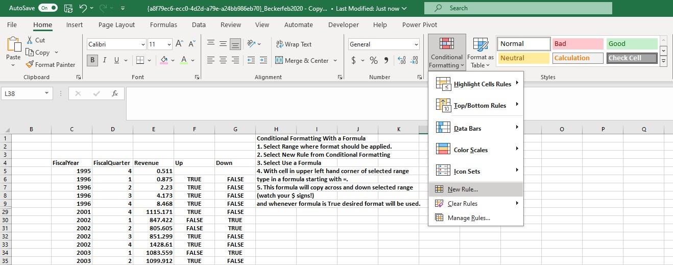
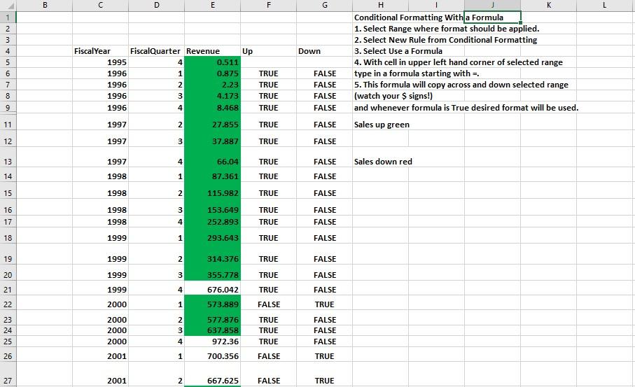
A new window will pop up, NEW FORMATTING RULE, and from there, you would choose USE A FORMULA TO DETERMINE WHICH CELLS TO FORMAT from the list. In the box titled FORMAT VALUES WHERE THIS FORMULA IS TRUE, we will enter E6>E5 and choose the FORMAT box. We want to highlight this green and will choose the color to reflect that. Finally, we will click OK.
Note in column F and G the row of TRUE and FALSE. This ensures that any cell in column E that is larger than its preceding cell will automatically highlight green also. Therefore, we fill in the Select a Rule Type dialog box as =E6>E6. After clicking OK, all revenues that were larger than the previous quarter are highlighted in green.
We want to format cell E6 in red if E6<E5. If this formula is copied down then whenever the formula is True (see Column G, we should format the quarter’s revenue in green. We can also add a new rule following the same format, where we add the formula =EE6<E5 and choose to format the applicable cells with a red highlight.
As shown below, the revenues that were larger than the previous quarter are highlighted in green and the revenues that were smaller than the previous quarter are highlighted in red.
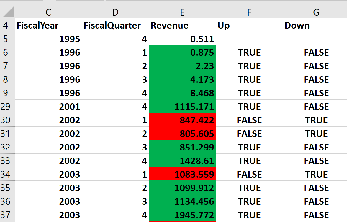
Figure 4 Revenue increases are highlighted in Green and Revenue decreases are highlighted in Red.
Note that Column E is highlighted in Green if and only if Column F contains TRUE Green and Column E is highlighted in Red if and only if Column G contains TRUE.
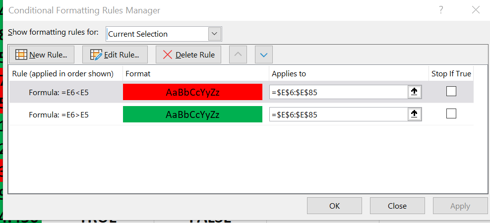
If your cursor is anywhere in the range (E6:E85) where the format was applied, selecting Manage Rules from the Conditional Formatting menu will show you the conditional formats (see Figure 5) applied to that range.
Learn how to use more automation features with our free Excel ebook!
Conditional formatting is just one way to save time when working in Excel! Download our free ebook, Excel Essentials for Accountants: Boosting Productivity and Accuracy with Automation and learn how to apply a variety of functions, create pivot tables, record a macro in Excel, and so much more!